6.5.1 Simple probability valuation techniques
The most simple risk valuation technique is a subjective assessment of probability for each risk. This approach has the advantage that it is easier to construct and interpret than advanced statistical methods.
Subjective assessments should, where possible, be based on past experience, current best practice and likely improvements in the future, supported by reliable information where available. Typically this will involve analysis of the same information used to identify the consequences of risk to observe the extent and frequency of time and cost overruns in previous similar projects.
One of these techniques is the point estimate approach. Practitioners should realistically assess how likely final costs are to be above, or below the amount included in the Raw PSC. The number of point estimates used in valuing risk (each having a different expected consequence) should reflect the materiality of the risk and the information available.
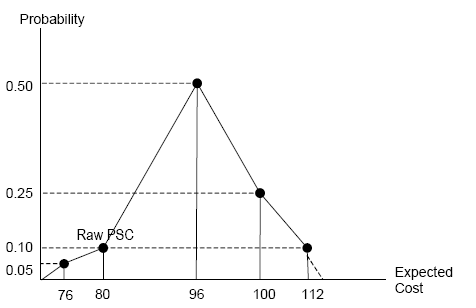
Figure 6-4 illustrates the point estimate approach for the construction risk associated with a hypothetical water treatment plant, presented as a simple probability distribution.
Figure 6-4 Hypothetical probability distribution (point estimate approach)
Example 1 provides a simple example using a point estimate approach
Example 1 Construction risk (simple case) |
Consider the construction of a water treatment plant with a base NPC capital cost of $80 million (this is the amount included in the Raw PSC) over a two-year construction period. Evidence in similar public procurement projects suggests that there is only a 10 per cent probability that actual construction costs (including both cost and time overrun) will be the same as the initial base amount included in the Raw PSC (a risk consequence of $0.0 million), while the most likely outcome is expected to exceed the initial base amount by around 20 per cent (a 'likely' over run of $16 million). It is also estimated that there is a further risk of a 25 per cent increase (a 'moderate' over run of $20 million), and a smaller risk that costs will increase by up to 40 per cent (an 'extreme' over run of $32 million). In addition, there is a further possibility that costs may actually be 5 per cent below the base amount (a consequence of $-4.0 million, representing the potential reduction in cost). This can be summarised into the following table (assume the probabilities are given - estimating the probability of the consequence of risk occurring is covered in Section 6.5). |
Scenario | Outcome ($m) | Consequence ($m) | Probability | Value of risk ($m) | ||
Below the base amount | 76.0 | -4.0 | 0.05 | -0.2 | ||
No overrun | 80.0 | 0.0 | 0.10 | 0.0 | ||
Overrun: likely | 96.0 | 16.0 | 0.50 | 8.0 | ||
Overrun: moderate | 100.0 | 20.0 | 0.25 | 5.0 | ||
Overrun: extreme | 112.0 | 32.0 | 0.10 | 3.2 | ||
Total: 16.0 |
When assessing the consequence of risk, the expected timing of the cash flows also needs to be considered (a) to account for the effect of the discount rate, and (b) to convert to nominal cash flows (to include the effect of inflation). The timing of the impact of construction risk generally occurs during and slightly after the construction period, depending on the likelihood of time over runs. If 70 per cent of the risk (valued above) is assumed to be expected during initial construction in Year 0, with the remaining 30 per cent in Year 1, the cash flows associated with the risk could be represented as follows (note for simplicity this assumes all cash flows occur at the beginning of the period): |
Cost | Year 0 ($m) | Year 1 ($m) | ||
Construction risk |
| |||
Real cost | 11.2 | 4.8 | ||
Nominal cost | 11.2 | 4.9 | ||
(assume inflation @ 2.5% p.a.) | ||||
Discount factor (assume discount rate @ 8.65% p.a.) | ||||
1.00 | 1.09 | |||
Discounted cash flows | 11.2 | 4.5 | ||
Present value | 15.7 |
The present value of construction risk in this example would be $15.7 million, equivalent to approximately 19.7 per cent of the construction cost included in the Raw PSC. |